Solving the "Beautiful Bridges" Problem, Algebraically

Beautiful Bridges is one of the eleven problems in ACM ICPC World Finals 2019. The problem set can be found here. In this post, we are going to solve this problem in two different ways, both of which involve specifying the problem as a relational hylomorphism, and extracting, via algebraic reasoning, an efficient functional program that conforms to the specification.

Basic knowledge of category theory and recursion schemes would be helpful for following the post. Nothing fancy is required.

Motivation

First of all, why do we want to do this? What’s the point?

There are at least two reasons:

First, algebraic methods give us a more mathematical, and more abstract way of solving problems. This can be very enlightening, since by abstracting away the details, we have a much better view of the essence of the problem, and the commonality of different problems. In fact, I would argue that this does not only benefit programming, but is good advice for life in general. When we try to view the problems we have in our lives in a more abstract way, it helps us see the big pictures better, make better decisions, and avoid getting caught up in the details.

When programmers need to solve a programming task, many of them do so based on the knowledge they were taught and their experiences, and come up with a solution in a fairly ad-hoc way that is hard to describe rigorously or generalize. And there’s nothing terribly wrong with that; after all the ultimate goal is to solve the problems. But ideally, in my opinion, solving programming problems should be more structured, more scientific, and less ad-hoc than that.

Second, for certain problems, solving them via algebraic methods could be easier than solving them directly. Algebraic reasoning is far from straightforward, but a nice thing is that once we’ve come up with a relational specification of the problem, the task of deriving a functional program from the specification is often a relatively mechanical one. While it is rarely so mechanical that the derivation can be done completely automatically, it is definitely possible to take advantage of a proof assistant, such as Agda or Coq, or a relational/logic programming library, to facilitate the derivation. You will certainly need to guide the proof assistant or the relational/logic programming library, but they may be able to tell you what the remaining obstacles are that you need to clear, and may automatically generate solutions/proofs to some relatively simple sub-problems. Examples of such libraries include AoPA, Barliman and Edward Kmett’s guanxi. It is conceivable that these libraries will become more and more powerful in the near future, and make the lives of programmers easier and easier.

Coming up with a relational specification of the problem is usually not terribly hard either. Due to the expressive power of relational calculus (relations are generalization of functions and are quite expressive), it is often fairly natural to specify a problem using relations and relational operators.

As a simple example, the function permute :: [a] -> Set [a], which generates all permutations of a list, can simply be specified as

permute = Λ (bagify° . bagify)

where:

• bagify :: List -> Bag is a relation that relates lists with bags (i.e. multisets). A pair (list, bag) is related by bagify if they contain the same elements (i.e., the bag simply forgets the order of elements in the list).
• R° is the converse of R. Thus bagify° . bagify is a relation that relates two lists. Two lists are related by bagify° . bagify iff they are related to the same bag, i.e., one is a permutation of the other.
• Λ is the power transpose operator, also known as the breadth operator. It converts a relation of type a -> b into a function of type a -> Set b, which, for each a, returns the set of bs related to a by the relation.

Any specification or implementation of permute using functions is bound to be longer and more involved than the above relational specification.

Preliminaries

Relations and Allegories

Relations are generalization of functions. A relation between A and B may map each a ∈ A to a single b ∈ B, no b at all (which partial functions also allow), or multiple bs (which partial functions do not allow). Thus a relation can be viewed as a subset of the cartesian product of A and B, and the converse (which some authors call reciprocation) of a relation R is also a relation, denoted by R°. We use a R b to denote that a and b are related by relation R :: A -> B.

Allegories are generalization of categories. Arrows with the same source and target are equipped with a partial order ⊆, called inclusion. For any two arrows R, S :: A -> B, there is an arrow R ∩ S :: A -> B, called the meet of R and S. In lattice theory terminology, every (locally-small) allegory is locally a meet-semilattice.

Relators are generalization of functors. A relator F is a mapping between two allegories, which satisfies all functor laws, plus monotonicity:

R ⊆ S ⟹ F R ⊆ F S

for all relations R and S.

The composition of two relations, R :: B -> C and S :: A -> B, is a relation R . S :: A -> C defined as

a (R . S) c  ≡  ∃b. a S b  and  b R c

There are laws associated with some of the operators introduced above, such as converse and inclusion, but we omit them since they are not important for the topic of this post.

By convention, a single upper case letter usually denotes relations, functors and relators, and a single lower case letter functions and sets/types.

Pair Calculus

The pair calculus introduces the following useful operators:

• The fork operator, △, turns relations R :: a -> b and S :: a -> c, into R △ S :: a -> b × c (× is defined below).
• The join operator, ▽, turns relations R :: a -> c and S :: b -> c, into R ▽ S :: a + b -> c (+ is defined below).
• The product operator, ×, turns sets a and b into their cartesian product: a × b = (a,b), and turns relations R :: a -> c and S :: b -> d into R × S :: (a,b) -> (c,d), defined as R × S = R . fst △ S . snd.
• The coproduct operator, +, turns sets a and b into their disjoint union: a + b = Either a b, and turns relations R :: a -> c and S :: b -> d into R + S :: Either a b -> Either c d, defined as R + S = Left . R ▽ Right . S.

It is worth mentioning that cartesian product a × b is not a categorical product in the category of sets and relations, where both the categorical product and the categorical coproduct of a and b is a + b. Thus a × b is often referred to as the relational product to distinguish it from the categorical product.

To reduce the number of parentheses, we assign the lowest precedence to ▽. For example, R . S ▽ U ∪ V = (R . S) ▽ (U ∪ V). Note that this is not the case in some of the literature.

Recursion Schemes

I’m assuming the readers have basic knowledge of recursion schemes, such as reasonable familiarity with the concepts of catamorphisms, anamorphisms, hylomorphisms, algebra, coalgebra, etc. I’ll briefly describe them below, but this post would be way too long if I have to explain the basics.

The following figure shows the commuting diagrams of catamorphisms and anamorphisms:

Here F is a base functor (also called pattern functor or shape functor); Mu F and Nu F are the least and greatest fixed points of F, respectively; embed and project are the initial algebra and the final coalgebra of F, respectively. Both catamorphisms and anamorphisms can be generalized to relations: when R is a relation, F becomes a relator, and cata R and ana R become relational catamorphism and anamorphism.

A nice thing about relations, and in particular relators, is that the least fixed point, Mu F, and the greatest fixed point Nu F of any “normal” relator F coincide, which we call Fix F. This makes sense, because the converse of a relation is still a relation, so if we reverse all arrows in the catamorphism diagram, it becomes the anamorphism diagram. This means catamorphisms can be composed with anamorphisms to form hylomorphisms, as shown below.

It is not in general the case that Mu F and Nu F coincide. For instance, in the category Set (sets and total functions), let ListF a be the base functor of cons-lists whose elements are of type a, then Mu (ListF a) is finite lists (which is the carrier of the initial algebra of ListF a), while Nu (ListF a) is possibly infinite lists (which is the carrier of the final coalgebra of ListF a). Thus catamorphisms and anamorphisms are not composable, and there are no hylomorphisms. In Haskell, though, loosely speaking, least fixed points and greatest fixed points for functors do coincide.

Another nice thing about relations is that we don’t really need the concept of anamorphism, because an anamorphism is just the converse of a catamorphism:

ana R = (cata R°)°

Therefore a relational hylomorphism is in the form of cata S . (cata T)°. This is nice since we don’t need to remember the laws and theorems for anamorphisms. We can just use the laws and theorems for catamorphisms and converse in our algebraic reasoning. In the rest of the post we’ll denote cata R as ⦇R⦈.

A Brief Overview of the Problem

The function we need to construct to solve the Beautiful Bridges problem has the following type:

beautifulBridges :: [(Int, Int)] -> Int -> Int -> Int -> Maybe Int

The first argument, [(Int, Int)], is the ground profile, and is guaranteed to contain at least two elements. Each (Int, Int) is the position of a key point, on which a pillar may be built. The other three arguments are h, α and β. For simplicity, we assume that h, α and β are constants, so that the functions we define don’t need to take them as parameters. Furthermore, for convenience, we convert the list of key points into a non-empty list of segments, each of which represents a segment of the ground between two adjacent key points, by zipping it with its tail. Thus what we need to compute becomes

beautifulBridges :: Nel Segment -> Maybe Int

where

type Point = (Int, Int)
type Segment = (Point, Point)

Nel is non-empty cons-lists, and all catamorphisms in this post are on Nel. It is defined as

data Nel a = Wrap a | Cons a (Nel a)

The base functor of Nel is NelF, which can be viewed as a functor on b, or a bifunctor on a and b:

data NelF a b = WrapF a | ConsF a b

NelF can be characterized by its actions on objects and arrows:

NelF a b = a + a × b    -- action on objects (types)
NelF a R = id + id × R  -- action on arrows (relations)

Let wrap = Wrap and cons = uncurry Cons. Thus the initial algebra of NelF is wrap ▽ cons. Uncurried functions are often more useful in algebraic reasoning than their curried counterparts.

beautifulBridges returns the cost of the optimal bridge, or Nothing if no valid bridge exists. This problem is obviously decidable, since the number of possible bridges is finite and can be easily enumerated. It also has a fairly simple dynamic programming solution, but it takes O(n³) time. Most ICPC problems tell you the sizes of the test cases, from which one can usually infer the required time complexity of the solutions. For this problem, a test case has up to 10,000 segments. This indicates that we can’t afford anything O(n³) or above, and that a correct solution is likely an O(n²) or an O(n²logn) one.

For optimization problems like this one, a viable approach is to specify the problem as the power transpose of a relational hylomorphism, followed by a min operator:

min R . Λ (⦇S⦈ . ⦇T⦈°)

where min is specified as:

-- returns a minimum element of the set wrt R, if exists, breaking ties arbitrarily.
min :: (a -> a) -> Set a -> a
xs (min R) x  ⟹  x ∈ xs  and  ∀ y ∈ xs. y R x

This form of specification is quite general, and captures a large class of optimization problems. ⦇T⦈° generates intermediate structures, or subproblems, ⦇S⦈ combines the solutions to the subproblems, and min R takes the optimal solution.

There are two commonly used special cases of the above specification:

• T is the initial algebra, hence ⦇T⦈ = id, and so the specification becomes

  min R . Λ ⦇S⦈
  

  This is the case when we already have the “intermediate” structure to begin with.

• S is a function. Denote it by h, we have

  min R . Λ (⦇h⦈ . ⦇T⦈°)
  

We are going to discuss both of these options for Beautiful Bridges. The first option, where ⦇T⦈ = id, leads to a thinning approach, and the second option, where S = h, leads to a dynamic programming approach.

Thinning

Specification

The Beautiful Bridges problem can be specified as

beautifulBridges ⊆ fmap cost . setToMaybe . Λ (min R . Λ (ok? . partition))

where

type Arch = Nel Segment  -- An arch is a non-empty list of segments
type Bridge = Nel Arch   -- A bridge is a non-empty list of arches

-- 'partition' is a relation that relates a list with a partition of it.
-- It is the converse of 'concat'.
partition :: Nel a -> Nel (Nel a)
partition = concat°

-- 'concat' is a function that returns the concatenation of a list of lists.
-- It is a (functional) catamorphism.
concat :: Nel (Nel a) -> Nel a
concat = ⦇id ▽ cat⦈

-- 'cat' concatenates two lists. cat = uncurry (<>).
cat :: (Nel a, Nel a) -> Nel a

-- 'ok?' is a (coreflexive) relation that takes a bridge, and returns
-- back the same bridge if it is valid, otherwise it returns nothing.
ok? :: Bridge -> Bridge

-- bridge1 R bridge2 iff the cost of bridge1 is no more than that of bridge2.
-- cost :: Bridge -> Int returns the cost of a bridge.
-- x leq y iff x <= y.
R :: Bridge -> Bridge
R = cost° . leq . cost

-- setToMaybe = Data.Set.lookupMin
setToMaybe :: Set a -> Maybe a

A relation S ⊆ id, such as ok?, is called a coreflexive or a predicate. If S is a coreflexive, then S = S°. Coreflexives are marked by a ? in the end. For a coreflexive p? :: a -> a, its corresponding Boolean-valued function, p :: a -> Bool, maps a to True iff a p? a. Conversely, any Boolean-valued function p can be turned into a coreflexive p?.

The specification says that the behavior of beautifulBridges is that it first partitions the given list of segments in all possible ways (each representing a different way to build a bridge), and keeps the valid bridges (ok?), then takes the optimal bridge (min R), if any. The outer Λ operator then converts it into a Set that is either empty (if no valid bridge exists) or contains exactly one element. The Set is then turned into a Maybe, and the optimal bridge is converted into its cost.

Note that the specification above uses ⊆ as opposed to =. For this problem it doesn’t matter, because the rhs is a function. For any two functions f and g, f ⊆ g is equivalent to f = g. It is sometimes the case that the rhs is a relation that needs to be refined down to a function, hence ⊆ is commonly used in relational specifications.

The above specification is slightly complicated by the fact that there may not exist a valid bridge, and the requirement to return the cost of the optimal bridge, if exists. If a valid bridge is guaranteed to exist, and the requirement is to return the optimal bridge itself (rather than its cost), the rhs of the above specification would simply be min R . Λ (ok? . partition). Fortunately, the additional complication can pretty much be ignored in the derivation process.

To apply the theorems relevant to the construction of the thinning approach, we need to convert min R . Λ (ok? . partition) into the form min R . Λ ⦇S⦈, i.e., we need to specify ok? . partition as a catamorphism. This can be done in two steps:

1. Express partition as a catamorphism. partition is expressed above as the converse of a catamorphism, concat°. It can also be expressed directly as a catamorphism:

   partition = ⦇wrap . wrap ▽ new ∪ glue⦈
   

   where new, glue :: (a, Nel (Nel a)) -> Nel (Nel a); new creates a new partition for a and adds it to the front of the existing list of partitions, and glue adds a to the front of the first existing partition.

2. Appeal to the fusion law for catamorphisms to fuse ok? into the catamorphism.

The fusion law for catamorphisms reads

T . F S ⊆ S . R  ⟹  ⦇T⦈ ⊆ S . ⦇R⦈
T . F S ⊇ S . R  ⟹  ⦇T⦈ ⊇ S . ⦇R⦈
T . F S = S . R  ⟹  ⦇T⦈ = S . ⦇R⦈

where F is the base relator of the catamorphism. For this problem, it turns out appealing to the fusion law directly doesn’t work, due to the following crucial observation: an invalid arch may be widened into a valid one.

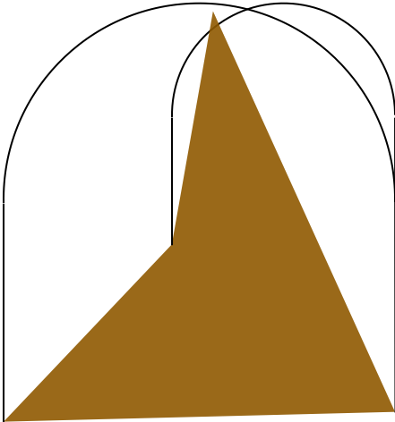
As shown in the graph above, the smaller arch is invalid, but we can widen it towards the left to form a valid larger arch. Therefore, we can’t simply discard all invalid arches; and so fusing ok? into the catamorphism, which means all intermediate bridges need to be valid, isn’t going to work.

To cope with this, we will split the predicate ok? into two predicates, okHead? and okTail?, such that

ok? = okHead? . okTail?

okHead holds for a bridge if the first arch is a valid arch; okTail holds for a bridge if the tail is a valid bridge. The idea is to fuse okTail? into the catamorphism, and incorporate okHead? in the definition of R. To do the latter, we can set the cost of a bridge to Nothing if okHead does not hold, or Just k if it holds and the cost of the bridge is k. Let cost' denote the modified cost function, and let R' = cost'° . leq . cost', under the assumption ∀k. (Just k) leq Nothing. Now the specification of beautifulBridges becomes

beautifulBridges ⊆ cost' . min R' . Λ(okTail? . partition)

As we can see by comparing this specification with the previous one, an additional benefit of splitting ok? into okHead? and okTail? is that the set returned by Λ(okTail? . partition) is guaranteed to contain at least one bridge, since okTail is vacuously true for the bridge with a single arch that spans all segments. Therefore we can simply apply cost' after min R'.

The task now is to fuse okTail? into the catamorphism, and obtain the following specification:

beautifulBridges ⊆ cost' . min R' . Λ ⦇S⦈

for some suitable S.

Since the catamorphism is on Nel, whose initial algebra is wrap ▽ cons, S must be in the form of U ▽ V for some U and V. Appealing to the fusion law, we need to find U and V such that

  (U ▽ V) . NelF okTail? = okTail? . (wrap . wrap ▽ new ∪ glue)
≡ { definition of NelF }
  (U ▽ V) . (id + id × okTail?) = okTail? . (wrap . wrap ▽ new ∪ glue)
≡ { coproduct fusion: ∀ R S U V: (R ▽ S) . (U + V) = R . U ▽ S . V }
  U ▽ V . (id × okTail?) = okTail? . (wrap . wrap ▽ new ∪ glue)
≡ { coproduct: ∀ R S U: U . (R ▽ S) = U . R ▽ U . S }
  U ▽ V . (id × okTail?) = okTail? . wrap . wrap ▽ okTail . (new ∪ glue)

The last equation follows from

U = okTail? . wrap . wrap = wrap . wrap  -- 'okTail' is vacuously true here
V . (id × okTail?) = okTail? . (new ∪ glue)

The first condition determines U. To obtain V, since the right hand side of the second condition contains new ∪ glue, we decompose V into V1 ∪ V2. Since composition distributes over join, it suffices to find V1 and V2 such that

V1 . (id × okTail?) = okTail? . new
V2 . (id × okTail?) = okTail? . glue

To construct V1, observe that okTail? is a catamorphism:

okTail? = ⦇wrap ▽ cons . (id × ok?)⦈

And so we reason

  okTail? = ⦇wrap ▽ cons . (id × ok)⦈
≡ { catamorphism }
  okTail? . (wrap ▽ cons) = (wrap ▽ cons . (id × ok?)) . (id + id × okTail?)
≡ { coproduct fusion }
  okTail? . wrap ▽ okTail . cons = wrap ▽ cons . (id × ok?) . (id × okTail?)
⟹ { coproduct cancellation }
  okTail? . cons = cons . (id × ok?) . (id × okTail?)
≡ { × preserves composition; ok? . okTail? = ok? }
  okTail? . cons = cons . (id × ok?)
≡ { composition }
  okTail? . cons . (wrap × id) = cons . (id × ok?) . (wrap × id)
≡ { definition of new }
  okTail? . new = cons . (id × ok?) . (wrap × id)
≡ { × preserves composition }
  okTail? . new = cons . (wrap × id) . (id × ok?)
≡ { definition of new }
  okTail? . new = new . (id × ok?)
≡ { id = id . id; ok? = okHead? . okTail? }
  okTail? . new = new . ((id . id) × (okHead? . okTail?))
≡ { × preserves composition }
  okTail? . new = new . (id × okHead?) . (id × okTail?)
≡ { let V1 = new . (id × okHead?) }
  okTail? . new = V1 . (id × okTail?)

where “× preserves composition” refers to the following law

(R × S) . (U × V) = (R . S) × (U . V)

Thus we have V1 = new . (id × okHead?).

In a similar way we can show that V2 = glue.

All in all, we have converted the specification into one of the canonical forms, i.e., power transpose of a catamorphism followed by a min operator:

beautifulBridges ⊆ cost' . min R' . Λ ⦇wrap . wrap ▽ (new . (id × okHead?)) ∪ glue⦈

Intuitively, we only allow adding a new arch via new, if the first arch is valid. This maintains the invariant that the tail of an intermediate bridge is always valid. On the other hand, we don’t impose any condition on glue: glueing a segment to the first arch is always allowed (this is not the optimal strategy and we’ll discuss the optimization in the end, but it doesn’t increase the time complexity).

The next step is to convert the above specification into an efficient implementation.

Derivation

Given a specification of the form min R . Λ ⦇S⦈, we always have the option of computing it directly using a brute-force approach. The brute-force approach is an application of the Eilenberg-Wright Lemma:

Λ ⦇S⦈ = ⦇Λ (S . F ∋)⦈

where ∋ :: Set a -> a is the membership relation that relates Set a with a, if the latter is a member of the former. It says that to compute Λ ⦇S⦈, we can move the power transpose, Λ, into the algebra of the catamorphism, i.e., compute all possible subsolutions at each step.

The catamorphism on the right hand side of the above equation is a functional catamorphism since the algebra is a function, and so it can be easily translated into a Haskell program. It of course runs in exponential time, which can’t possibly work, since the number of segments is up to 10,000 in the problem.

With the brute-force approach being a non-starter, the next simple thing to look for is the other extreme: whether a greedy solution exists. The Greedy Theorem states that for the greedy approach to work, we need to show that the algebra of the catamorphism is monotonic on R°. In our case, we need to show

(U ▽ V) . F R'° ⊆ R'° . (U ▽ V)

where U, V, F and R' are defined in the previous section.

In words, it says if we start with a worse subsolution, we always end up getting a worse solution (and therefore we can discard all such “worse subsolutions”). If we can prove that this holds, we can use the following inequation to derive a greedy approach:

⦇min R . ΛS⦈ ⊆ min R . Λ ⦇S⦈

That is, instead of taking min R in the end, we can take min R at each step in the catamorphism, and discard all other intermediate solutions. Unfortunately, the above condition obviously doesn’t hold for this problem. It is easy to see that a worse sub-bridge may lead to a better bridge, and a better sub-bridge may lead to a worse bridge, or may not lead to a valid bridge at all.

Therefore we need to do something in between brute-force and greedy, and one option is to use a thinning approach.

The thinning approach requires a refined ranking criteria Q, such that Q ⊆ R and our algebra is monotonic on Q°. If we can find such a Q, then the Thinning Theorem gives us

min R = min R . thin Q
⦇thin Q . Λ(S . F ∋)⦈ ⊆ thin Q . Λ ⦇S⦈

where thin Q discards a subsolution if there’s a better subsolution in terms of Q.

For our problem, there is a fairly intuitive choice of Q:

Q = R' ∩ (head° . head)

(head° . head) relates two bridges iff they have the same first arch, and thus Q basically says that a bridge is better than another in terms of Q if they have the same first arch, and the cost of the first bridge is smaller. The claim that the algebra is monotonic on Q° can be proved formally (details are omitted), and intuitively it also makes sense: it is easy to see that if a bridge is worse than another in terms of Q, then building more arches on the left or extending the leftmost arch towards the left can’t possibly lead to a better bridge. Therefore, at each step, rather than keeping only the single best bridge in terms of R as the greedy approach does, we keep all bridges for which there’s no better bridge in terms of Q. In other words, we keep the best bridge for each possible first arch.

There are also formal methods on how to extract an efficient implementation of thin Q, but in our case it’s fairly simple. In each step, the previous sub-bridges are already thinned, i.e., they all have distinct first arches. We perform both new . (id × okTail?) and glue; glue still results in distinct first arches, and new results in a number of new sub-bridges with the same first arch, so we just need to keep the lowest cost sub-bridges among all sub-bridges produced by new, if any.

This leads to the following approach for the Beautiful Bridges problem:

beautifulBridges = cost' . min R' . ⦇thin Q . Λ(S . F ∋)⦈

where, to repeat the definitions obtained before,

S = U ▽ V
U = wrap . wrap
V = V1 ∪ V2
V1 = new . (id × okHead?)
V2 = glue
Q = R' ∩ (head° . head)
R' = cost'° . leq . cost'
F R = id + id × R

At each step, given the new segment and the list of previous subsolutions, for each subsolution (picked by ∋), it generates a new bridge by extending the first arch of the bridge to include the new segment (i.e., glue, via V2); and if the first arch of the bridge is a valid arch, it generates another new bridge by creating a new arch (i.e., new, via V1). In the very first step, it simply wraps the first segment into a bridge (via U). Finally, it retains the best bridge created via new, along with all bridges created via glue, as the set of subsolutions for the next step (i.e., thin Q).

Since checking the validity of an arch naively takes O(m) time where m is the number of segments included in an arch, a naive implementation of this approach still takes O(n³) time. We will discuss later how to reduce it to O(n²) time.

The implementation of the thinning solution can be found here.

Dynamic Programming

Specification

We now turn our attention to the alternative specification of Beautiful Bridges, as the converse of a relational catamorphism:

beautifulBridges ⊆ fmap cost . setToMaybe . Λ (min R . Λ (ok? . ⦇id ▽ cat⦈°))

The dynamic programming theorems depend on the algebra of the catamorphism, i.e., h in min R . Λ (⦇h⦈ . ⦇T⦈°), being a function, but ok? is a relation (in particular, a coreflexive). There are multiple resolutions:

• Turn ok? into a Maybe valued functional catamorphism, and modify the definition of R to accommodate it,
• Appeal to the fusion law to fuse ok? into concat°.
• Modify the cost function such that invalid bridges have infinite costs, possibly represented by Nothing.
• Express ok? as a catamorphism, and appeal to the fusion law to fuse concat° into ok?.

We’ll go with the last option above since it appears to be the simplest.

Since ok? is a coreflexive, we have ok? = ok?°. If we can express ok? as a catamorphism, ok? = ⦇H⦈, then we have

  ⦇T⦈° = ok? . concat°
≡ { converse: ∀ R S: (R . S)° = S° . R°; ok? = ok?° }
  ⦇T⦈ = concat . ok?
≡ { ok? = ⦇H⦈ }
  ⦇T⦈ = concat . ⦇H⦈
⟸ { fusion }
  T . F concat = concat . H

(⟸ is pronounced “follows from”)

And ok? can indeed be written as a catamorphism:

ok? = ⦇wrap . okArch? ▽ cons . (okArch? × id)⦈

where okArch? :: Arch -> Arch is a coreflexive that holds if the arch is valid. Since T is an algebra for functor NelF, we have T = U ▽ V for some U and V. Based on T . F concat = concat . H, U and V should satisfy:

U = concat . wrap . okArch?
V . (id × concat) = concat . cons . (okArch? × id)

The first equation determines U: since concat . wrap = id, we have U = okArch?. To construct V, we reason:

  V . (id × concat) = concat . cons . (okArch? × id)
≡ { concat = ⦇id ▽ cat⦈ }
  V . (id × concat) = cat . (id × concat) . (okArch? × id)
≡ { × preserves composition }
  V . (id × concat) = cat . (okArch? × id) . (id × concat)
⟸
  V = cat . (okArch? × id)

So now the specification of the problem becomes

beautifulBridges ⊆ fmap cost . setToMaybe . Λ (min R . Λ ⦇okArch? ▽ cat . (okArch? × id)⦈°)

Derivation

For the dynamic programming approach to work, the condition is that h, the algebra of the catamorphism, should be monotonic on R. In this case ⦇h⦈ = id = ⦇wrap ▽ cons⦈, so we need to show that

(wrap ▽ cons) . F R ⊆ R . (wrap ▽ cons)

This says if we first take a better bridge, and add an arch to it, we can also first add an arch, then take a better bridge. This is obviously true, since the condition does not say anything about the validity of the bridge.

According to the Dynamic Programming Theorem, if h is monotonic on R, then

min R . Λ ⦇okArch? ▽ cat . (okArch? × id)⦈°

can be obtained by computing the least fixed point of the recursion equation

X = min R . fmap ((wrap ▽ cons) . (id + id × X)) . Λ (okArch? ▽ cat . (okArch? × id))°

where the fmap has type (a -> b) -> Set a -> Set b. Note that the (a -> b) in the type is a relation: given an a it may not return a b, since given a number of consecutive segments, there may not exist a valid bridge that can be built on these segments.

The Λ(...)° part unfolds the current subproblem to create the next layer of subproblems; the fmap (...) part recursively solves these subproblems; and min R takes the optimal solution. Intuitively, this is exactly how dynamic programming works (minus tabulation/memoization).

In the following I’ll explain the intuition of extracting the functional program and omit the formal derivation.

Λ(okArch? ▽ cat . (okArch? × id))° can be easily turned into a function: given xs = Nel Segment, it outputs Left xs if okArch xs, and Right (ys, zs) for all (ys, zs) such that ys ++ zs = xs and okArch ys.

Note that the set returned by Λ(okArch? ▽ cat . (okArch? × id))° is possibly empty. One way to deal with the empty set is to turn min R into a Maybe-valued function that returns Nothing if the input is an empty set. This allows us to express the entire X above as a Maybe-valued function. The remainder of the specification, fmap cost . setToMaybe . Λ, is straightforward.

For the dynamic programming solution to be efficient, one has to employ either tabulation (solving smaller subproblems first, and storing their results to speed up solving larger subproblems) or memoization (solving larger problems first, which recursively solves smaller problems, whose solutions are memoized). Haskell’s lazy evaluation is very convenient for memoization, and dynamic programming algorithms implemented in Haskell are usually shorter and more elegant than their counterparts in other programming languages. The readers are encouraged to check out my former coworker Travis Athougies’ blog post on this topic.

The implementation of the dynamic programming solution can be found here.

Optimization

As mentioned before, in a naive implementation, determining the validity of an arch that has m segments takes O(m) time. To improve the efficiency of this task, we can compute the validity of an arch incrementally. Suppose we use an algorithm that involves widening arches towards the left. The observation is that for any arch, if the left half of the arch intersects with the ground (such as the one shown in the figure above), it means the arch is too small, and needs to be extended to the left to form a valid arch. On the other hand, if the right half of the arch intersects with the ground, it means the arch is too big, and further extending it to the left cannot possibly lead to a valid arch.

Therefore, we can associate with each arch a minimum diameter and a maximum diameter. An arch whose diameter is within [minimum diameter, maximum diameter] is valid. When we extend an arch to the left by adding one more segment to it, we can update the minimum and maximum diameter in O(1) time, and thus determine the validity in O(1). This can be applied to both the thinning solution and the dynamic programming solution to bring down the complexity from O(n³) to O(n²).

Furthermore, If an arch’s diameter exceeds the maximum diameter, or if the minimum diameter exceeds the maximum diameter, there’s no need to further extend it to the left since it can’t possibly lead to a valid arch. In the thinning solution, recall that glueing a segment to the first arch is always allowed. We can make it more efficient by only allowing the glueing if the arch’s diameter has not exceeded its maximum diameter, and its minimum diameter has not exceeded its maximum diameter.

The details of computing the minimum and maximum diameters are left to the readers. Hint: it involves solving a simple quadratic equation.

Discussion

Both the thinning solution and the dynamic programming solution have the same O(n²) time complexity (with optimization), though they explore the search space in different ways: the thinning solution maintains the optimal bridges for a suffix of segments, and uses it to compute the optimal bridges with one additional segment; the dynamic programming solution tries all possible first arches of the bridge, and recursively computes the optimal tails.

For a problem that has both a thinning solution and a dynamic programming solution, it is in general not the case that both solutions have the same complexity. One example is the knapsack problem, where the dynamic programming solution takes pseudo-polynomial time and relies on the weights of items being integers, while the thinning solution, although taking exponential time in the worst case, does not rely on integer weights and is fairly efficient in practice.

Further Reading

• Algebra of Programming by Richard Bird and Oege De Moor
• Algebraic Methods for Optimization Problems by Richard Bird, Jeremy Gibbons and Shin-Cheng Mu